7 One Sample Inference

Now that you have all this information about descriptive statistics and probabilities, it is time to start inferential statistics. There are two branches of inferential statistics: hypothesis testing and confidence intervals.

Hypothesis Testing: making a decision about a parameter(s) based on a statistic(s).

Confidence Interval: estimating a parameter(s) based on a statistic(s).

This chapter will describe hypothesis testing, but as was stated in Chapter 1, the American Statistical Association (ASA) is suggesting not discussing statistical significance and p-values. So this chapter is mostly for background to understand previously published studies.

7.1 Basics of Hypothesis Testing

To understand the process of a hypothesis tests, you need to first have an understanding of what a hypothesis is, which is an educated guess about a parameter. Once you have the hypothesis, you collect data and use the data to make a determination to see if there is enough evidence to show that the hypothesis is true. However, in hypothesis testing you actually assume something else is true, and then you look at your data to see how likely it is to get an event that your data demonstrates with that assumption. If the event is very unusual, then you might think that your assumption is actually false. If you are able to say this assumption is false, then your hypothesis must be true. This is known as a proof by contradiction. You assume the opposite of your hypothesis is true and show that it can’t be true. If this happens, then your hypothesis must be true. All hypothesis tests go through the same process. Once you have the process down, then the concept is much easier. It is easier to see the process by looking at an example. Concepts that are needed will be detailed in this example.

7.1.1 Example: Basics of Hypothesis Testing

Suppose a manufacturer of the XJ35 battery claims the mean life of the battery is 500 days with a standard deviation of 25 days. You are the buyer of this battery and you think this claim is incorrect. You would like to test your belief because without a good reason you can’t get out of your contract.

7.1.1.1 Solution

What do you do?

Well first, you should know what you are trying to measure. Define the random variable.

Let $x$ = life of a XJ35 battery

Now you are not just trying to find different $x$ values. You are trying to find what the true mean is. Since you are trying to find it, it must be unknown. You don’t think it is 500 days. If you did, you wouldn’t be doing any testing. The true mean, $\mu$, is unknown. That means you should define that too.

Let $\mu$ = mean life of a XJ35 battery

Now what?

You may want to collect a sample. What kind of sample?

You could ask the manufacturers to give you batteries, but there is a chance that there could be some bias in the batteries they pick. To reduce the chance of bias, it is best to take a random sample.

How big should the sample be?

A sample of size 30 or more means that you can use the central limit theorem. Pick a sample of size 50.

Table 7.1 contains the data for the sample you collected:

Battery<- read.csv( "https://krkozak.github.io/MAT160/battery.csv") 
knitr::kable(head(Battery))

Table 7.1: Data on Battery Life
life
491
485
503
492
482
490

Now what should you do? Looking at the data set, you see some of the times are above 500 and some are below. But looking at all of the numbers is too difficult. It might be helpful to calculate the mean for this sample.

df_stats(~life, data=Battery, mean)

  response mean
1     life  490

The sample mean is 491.42 days. Looking at the sample mean, one might think that you are right. However, the standard deviation and the sample size also plays a role, so maybe you are wrong.

Before going any farther, it is time to formalize a few definitions.

You have a guess that the mean life of a battery is not 500 days. This is opposed to what the manufacturer claims. There really are two hypotheses, which are just guesses here — the one that the manufacturer claims and the one that you believe. It is helpful to have names for them.

Null Hypothesis: historical value, claim, or product specification. The symbol used is $H_o$.

Alternate Hypothesis: what you want to prove. This is what you want to accept as true when you reject the null hypothesis. There are two symbols that are commonly used for the alternative hypothesis: $H_a$ or $H_1$. The symbol $H_a$ will be used in this book.

In general, the hypotheses look something like this:

$H_0:\mu=\mu_o$

$H_a:\mu\ne \mu_o$

where $\mu_o$ just represents the value that the claim says the population mean is actually equal to.

Also, $H_a$ can be less than, greater than, or not equal to, though not equal to is more common these days.

For this problem:

$H_o:\mu=500\text{ days}$, since the manufacturer says the mean life of a battery is 500 days.

$H_a:\mu\ne 500\text{ days}$, since you believe that the mean life of the battery is not 500 days.

Now back to the mean. You have a sample mean of 491.42 days. Is this different enough to believe that you are right and the manufacturer is wrong? How different does it have to be?

If you calculated a sample mean of 235 or 690, you would definitely believe the population mean is not 500. But even if you had a sample mean of 435 or 575 you would probably believe that the true mean was not 500. What about 475? or 535? Or 483? or 514? There is some point where you would stop being so sure that the population mean is not 500. That point separates the values of where you are sure or pretty sure that the mean is not 500 from the area where you are not so sure. How do you find that point?

Well it depends on how much error you want to make. Of course you don’t want to make any errors, but unfortunately that is unavoidable in statistics. You need to figure out how much error you made with your sample. Take the sample mean, and find the probability of getting another sample mean less than it, assuming for the moment that the manufacturer is right. The idea behind this is that you want to know what is the chance that you could have come up with your sample mean even if the population mean really is 500 days.

Chances are probabilities. So you want to find the probability that the sample mean of 491.42 is unusual given that the population mean is really 500 days. To compute this probability, you need to know how the sample mean is distributed. Since the sample size is at least 30, then you know the sample mean is approximately normally distributed. Now, you want to find the $z$-value. The $z$-value is $z=\frac{491.42-500}{\frac{25}{\sqrt{50}}}=-2.43$.

This is more than 2 standard deviations below the mean, so that seems that the sample mean is usual. It might be helpful to find the probability though. Since you are saying that the sample mean is different from 500 days, then you are asking if it is greater than or less than. This means that you are in the tails of the normal curve. So the probability you want to find is the probability being more than 2.43 or less than $-2.43$. This is $P(-2.43<z)+P(z>2.43)=0.015$

pnorm(-2.43, 0, 1, lower.tail=TRUE)+pnorm(2.43, 0, 1, lower.tail=FALSE)

[1] 0.01509882

So the probability of being in the tails is 0.015. This probability is known as a p-value for probability-value. This is unusual, so it is unlikely to get a sample mean of 491.42 if the population mean is 500 days.

So it appears the assumption that the population mean is 500 days is wrong, and you can reject the manufacturer’s claim.

But how do you quantify really small? Is 5% or 10% or 15% really small? How do you decide?

Before you answer that question, a couple more definitions are needed.

Test statistic: $z=\frac{\bar{x}-\mu_o}{\frac{\sigma}{\sqrt{n}}}$ since it is calculated as part of the testing of the hypothesis

p - value: probability that the test statistic will take on more extreme values than the observed test statistic, given that the null hypothesis is true. It is the probability that was calculated above.

Now, how small is small enough? To answer that, you really want to know the types of errors you can make.

There are actually only two errors that can be made. The first error is if you say that is false, when in fact it is true. This means you reject when was true. The second error is if you say that is true, when in fact it is false. This means you fail to reject when is false. The following table organizes this for you:

7.1.2 Type of errors:

Type of errors
	Ho true	Ho false
Reject Ho	Type I error	no error
Fail to reject Ho	no error	Type II error

Thus

Type I Error is rejecting $H_o$ when $H_o$ is true, and

Type II Error is failing to reject $H_o$ when is $H_o$ false.

Since these are the errors, then one can define the probabilities attached to each error.

$\alpha$= P(type I error) = P(rejecting$H_o$ given it is true)

$\beta$= P(type II error) = P(failing to reject$H_o$ given it is false)

$\alpha$ is also called the level of significance.

Another common concept that is used is Power = $1-\beta$

Now there is a relationship between $\alpha$ and $\beta$. They are not complements of each other. How are they related?

If $\alpha$ increases that means the chances of making a type I error will increase. It is more likely that a type I error will occur. It makes sense that you are less likely to make type II errors, only because you will be rejecting more often. You will be failing to reject less, and therefore, the chance of making a type II error will decrease. Thus, as $\alpha$ increases, $\beta$ will decrease, and vice versa. That makes them seem like complements, but they aren’t complements. What gives? Consider one more factor -- sample size.

Consider if you have a larger sample that is representative of the population, then it makes sense that you have more accuracy then with a smaller sample. Think of it this way, which would you trust more, a sample mean of 490 if you had a sample size of 35 or sample size of 350 (assuming a representative sample)? Of course the 350 because there are more data points and so more accuracy. If you are more accurate, then there is less chance that you will make any error. By increasing the sample size of a representative sample, you decrease both $\alpha$ and $\beta$.

Summary of all of this:

For a certain sample size, $\alpha$ increases, $\beta$ decreases.
For a certain level of significance, $\alpha$, if $n$ increases, $\beta$ decreases.

Now how do you find $\alpha$ and $\beta$? Well $\alpha$ is actually chosen. There are only two values that are usually picked for $\alpha$: 0.01 and 0.05. is very difficult to find $\beta$, so usually it isn’t found. If you want to make sure it is small you take as large of a sample as you can afford provided it is a representative sample. This is one use of the Power. You want to be small and the Power of the test is large. The Power word sounds good.

Which pick of $\alpha$ do you pick? Well that depends on what you are working on. Remember in this example you are the buyer who is trying to get out of a contract to buy these batteries. If you create a type I error, you said that the batteries are bad when they aren’t, most likely the manufacturer will sue you. You want to avoid this. You might pick $\alpha$ to be 0.01. This way you have a small chance of making a type I error. Of course this means you have more of a chance of making a type II error. No big deal right? What if the batteries are used in pacemakers and you tell the person that their pacemaker’s batteries are good for 500 days when they actually last less, that might be bad. If you make a type II error, you say that the batteries do last 500 days when they last less, then you have the possibility of killing someone. You certainly do not want to do this. In this case you might want to pick $\alpha$ as 0.05. If both errors are equally bad, then pick $\alpha$ as 0.05.

The above discussion is why the choice of depends on what you are researching. As the researcher, you are the one that needs to decide what level to use based on your analysis of the consequences of making each error is.

If a type I error is really bad, then pick $\alpha$= 0.01.

If a type II error is really bad, then pick $\alpha$= 0.05

If neither error is bad, or both are equally bad, then pick $\alpha$ = 0.05

Usually $\alpha$ is picked to be 0.05 in most cases.

The main thing is to always pick the $\alpha$ before you collect the data and start the test.

The above discussion was long, but it is really important information. If you don’t know what the errors of the test are about, then there really is no point in making conclusions with the tests. Make sure you understand what the two errors are and what the probabilities are for them.

Now it is time to go back to the example and put this all together. This is the basic structure of testing a hypothesis, usually called a hypothesis test. Since this one has a test statistic involving $z$, it is also called a $z$-test. And since there is only one sample, it is usually called a one-sample $z$-test.

7.1.3 Example: Battery Example Revisited.

Steps of a hypothesis test:

State the random variable and the parameter in words
State the null and alternative hypothesis and the level of significance
State and check the conditions for a hypothesis test
Find the sample statistic, test statistic, and p-value
Conclusion:
Interpretation:

7.1.3.1 Solution

State the random variable and the parameter in words

$x$ = life of battery

$\mu$ = mean life of a XJ35 battery

State the null and alternative hypothesis and the level of significance

$H_o:\mu=500$

$H_a:\mu\ne500$

$\alpha$ = 0.05 (from above discussion about consequences)

State and check the conditions for a hypothesis test

Every hypothesis has some conditions that be met to make sure that the results of the hypothesis are valid. The conditions are different for each test. This test has the following conditions.

A random sample of size $n$ is taken.

This occurred in this example, since it was stated that a random sample of 50 battery lives were taken.

The population standard deviation is known.

This is true, since it was given in the problem.

The sample size is at least 30 or the population of the random variable is normally distributed.

The sample size was 30, so this condition is met.

Find the sample statistic, test statistic, and p-value

The test statistic depends on how many samples there are, what parameter you are testing, and conditions that need to be checked. In this case, there is one sample and you are testing the mean. The conditions were checked above.

Sample statistic:

df_stats(~life, data=Battery, mean)

  response mean
1     life  490

Test statistic: The z-value is $z=\frac{491.42-400}{\frac{25}{\sqrt{n}}}=-2.43$.

p-value: $P(-2.43<z)+P(z>2.43)=0.015$

Conclusion:

Now what? Well, this p-value is 0.015. This is a lot smaller than the amount of error you would accept in the problem $\alpha$ = 0.05. That means that finding a sample mean less than 490 days is unusual to happen if is true. This should make you think that is not true. You should reject $H_o$.

In fact, in general:

Reject $H_o$ if the p-value $<\alpha$

Fail to reject $H_o$ if the p-value $\ge\alpha$.

Interpretation:

Since you rejected $H_o$, what does this mean in the real world? That it what goes in the interpretation. Since you rejected the claim by the manufacturer that the mean life of the batteries is 500 days, then you now can believe that your hypothesis was correct. In other words, there is enough evidence to support that the mean life of the battery is less than 500 days.

Now that you know that the batteries last less than 500 days, should you cancel the contract? Statistically, there is evidence that the batteries do not last as long as the manufacturer says they should. However, based on this sample there are only ten days less on average that the batteries last. There may not be practical significance in this case. Ten days do not seem like a large difference. In reality, if the batteries are used in pacemakers, then you would probably tell the patient to have the batteries replaced every year. You have a large buffer whether the batteries last 490 days or 500 days. It seems that it might not be worth it to break the contract over ten days. What if the 10 days was practically significant? Are there any other things you should consider? You might look at the business relationship with the manufacturer. You might also look at how much it would cost to find a new manufacturer. These are also questions to consider before making any changes. What this discussion should show you is that just because a hypothesis has statistical significance does not mean it has practical significance. The hypothesis test is just one part of a research process. There are other pieces that you need to consider.

That’s it. That is what a hypothesis test looks like. All hypothesis tests are done with the same six steps. Those general six steps are outlined below.

7.1.4 Steps for hypothesis test

State the random variable and the parameter in words. This is where you are defining what the unknowns are in this problem.

$x$ = random variable

$\mu$ = mean of random variable, if the parameter of interest is the mean. There are other parameters you can test, and you would use the appropriate symbol for that parameter.

State the null and alternative hypotheses and the level of significance

$H_o:\mu=\mu_o$, where $\mu_o$ is the known mean

$H_a:\mu\ne\mu_o$, You can replace $\ne$ with $<$ or $>$ but usually you use $\ne$

Also, state your level here.

State and check the conditions for a hypothesis test

Each hypothesis test has its own conditions. They will be stated when the different hypothesis tests are discussed.

Find the sample statistic, test statistic, and p-value

This depends on what parameter you are working with, how many samples, and the conditions of the test. Technology will be used to find the sample statistic, test statistic, and p-value.

Conclusion

This is where you write reject $H_o$ or fail to reject $H_o$. The rule is: if the p-value $<\alpha$, then reject $H_o$. If the p-value $\ge\alpha$, then fail to reject $H_o$

Interpretation

This is where you interpret in real world terms the conclusion to the test. The conclusion for a hypothesis test is that you either have enough evidence to support $H_a$, or you do not have enough evidence to support $H_a$.

Sorry, one more concept about the conclusion and interpretation. First, the conclusion is that you reject or you fail to reject $H_o$. Why was it said like this? It is because you never accept the null hypothesis. If you wanted to accept the null hypothesis, then why do the test in the first place? In the interpretation, you either have enough evidence to support $H_a$, or you do not have enough evidence to support $H_a$. You wouldn’t want to go to all this work and then find out you wanted to accept the claim. Why go through the trouble? You always want to have enough evidence to support the alternative hypothesis. Sometimes you can do that and sometimes you can’t. If you don’t have enough evidence to support $H_a$, it doesn’t mean you support the null hypothesis; it just means you can’t support the alternative hypothesis. Here is an example to demonstrate this.

7.1.5 Example: Conclusions in Hypothesis Tests

In the U.S. court system a jury trial could be set up as a hypothesis test. To really help you see how this works, let’s use OJ Simpson as an example. In the court system, a person is presumed innocent until he/she is proven guilty, and this is your null hypothesis. OJ Simpson was a football player in the 1970s. In 1994 his ex-wife and her friend were killed. OJ Simpson was accused of the crime, and in 1995 the case was tried. The prosecutors wanted to prove OJ was guilty of killing his wife and her friend, and that is the alternative hypothesis. In this case, a verdict of not guilty was given. That does not mean that he is innocent of this crime. It means there was not enough evidence to prove he was guilty. Many people believe that OJ was guilty of this crime, but the jury did not feel that the evidence presented was enough to show there was guilt. The verdict in a jury trial is always guilty or not guilty!

The same is true in a hypothesis test. There is either enough or not enough evidence to support the alternative hypothesis. It is not that you proved the null hypothesis true.

When identifying hypothesis, it is important to state your random variable and the appropriate parameter you want to make a decision about. If you count something, then the random variable is the number of whatever you counted. The parameter is the proportion of what you counted. If the random variable is something you measured, then the parameter is the mean of what you measured. (Note: there are other parameters you can calculate, and some analysis of those will be presented in later chapters.)

7.1.6 Example: Stating Hypotheses

Identify the hypotheses necessary to test the following statements:

The average salary of a teacher is different from \$30,000.
The proportion of students who like math is not 10%.
The average age of students in this class differs from 21.

7.1.6.1 Solution

The average salary of a teacher is different from \$30,000.

$x$ = salary of teacher

$\mu=$ mean salary of teacher

The guess is that $\mu\ne30000$ and that is the alternative hypothesis.

The null hypothesis has the same parameter and number with an equal sign.

$H_o:\mu=30000$ $H_a:\mu\ne30000$

The proportion of students who like math is not 10%.

$x$ = number of students who like math

$p$ = proportion of students who like math

The guess is that $p$ is not 0.10 and that is the alternative hypothesis. $H_a:p\ne0.10$ and the null hypothesis would be $H_o:p=0.10$

The average age of students in this class differs from 21.

$x$ = age of students in this class

$\mu$=mean age of students in this class

The guess is that $\mu\ne21$ and that is the alternative hypothesis. $H_a:\mu\ne21$ and the null hypothesis would be $H_o: \mu=21$

7.1.7 Example: Stating Type I and II Errors and Picking Level of Significance

The plant-breeding department at a major university developed a new hybrid raspberry plant called YumYum Berry. Based on research data, the claim is made that from the time shoots are planted 90 days on average are required to obtain the first berry with a standard deviation of 9.2 days. A corporation that is interested in marketing the product tests 60 shoots by planting them and recording the number of days before each plant produces its first berry. The sample mean is 92.3 days. The corporation wants to know if the mean number of days is more than the 90 days claimed. State the type I and type II errors in terms of this problem, consequences of each error, and state which level of significance to use.
A concern was raised in Australia that the percentage of deaths of Aboriginal prisoners was higher than the percent of deaths of non-indigenous prisoners, which is 0.27%. State the type I and type II errors in terms of this problem, consequences of each error, and state which level of significance to use.

7.1.7.1 Solution

The plant-breeding department at a major university developed a new hybrid raspberry plant called YumYum Berry. Based on research data, the claim is made that from the time shoots are planted 90 days on average are required to obtain the first berry with a standard deviation of 9.2 days. A corporation that is interested in marketing the product tests 60 shoots by planting them and recording the number of days before each plant produces its first berry. The sample mean is 92.3 days. The corporation wants to know if the mean number of days is more than the 90 days claimed. State the type I and type II errors in terms of this problem, consequences of each error, and state which level of significance to use.

$x$ = time to first berry for YumYum Berry plant

$\mu$= mean time to first berry for YumYum Berry plant

Type I Error: If the corporation does a type I error, then they will say that the plants take longer to produce than 90 days when they don’t. They probably will not want to market the plants if they think they will take longer. They will not market them even though in reality the plants do produce in 90 days. They may have loss of future earnings, but that is all.

Type II error: The corporation do not say that the plants take longer then 90 days to produce when they do take longer. Most likely they will market the plants. The plants will take longer, and so customers might get upset and then the company would get a bad reputation. This would be really bad for the company.

Level of significance: It appears that the corporation would not want to make a type II error. Pick a 5% level of significance, $\alpha=0.05$.

A concern was raised in Australia that the percentage of deaths of Aboriginal prisoners was higher than the percent of deaths of non-indigenous prisoners, which is 0.27%. State the type I and type II errors in terms of this problem, consequences of each error, and state which level of significance to use.

$x$ = number of Aboriginal prisoners who have died

$p$ = proportion of Aboriginal prisoners who have died

Type I error: Rejecting that the proportion of Aboriginal prisoners who died was 0.27%, when in fact it was 0.27%. This would mean you would say there is a problem when there isn’t one. You could anger the Aboriginal community, and spend time and energy researching something that isn’t a problem.

Type II error: Failing to reject that the proportion of Aboriginal prisoners who died was 0.27%, when in fact it is higher than 0.27%. This would mean that you wouldn’t think there was a problem with Aboriginal prisoners dying when there really is a problem. You risk causing deaths when there could be a way to avoid them.

Level of significance: It appears that both errors may be issues in this case. You wouldn’t want to anger the Aboriginal community when there isn’t an issue, and you wouldn’t want people to die when there may be a way to stop it. It may be best to pick a 5% level of significance, $\alpha=0.05$.

Hint -- hypothesis testing is really easy if you follow the same recipe every time. The only differences in the various problems are the conditions of the test and the test statistic you calculate so you can find the p-value. Do the same steps, in the same order, with the same words, every time and these problems become very easy.

7.1.8 Homework for Basics of Hypothesis Testing Section

For the problems in this section, a question is being asked. This is to help you understand what the hypotheses are. You are not to run any hypothesis tests nor come up with any conclusions in this section.

The Arizona Republic/Morrison/Cronkite News poll published on Monday, October 20, 2016, found 390 of the registered voters surveyed favor Proposition 205, which would legalize marijuana for adults. The statewide telephone poll surveyed 779 registered voters between Oct. 10 and Oct. 15. (Sanchez, 2016) Fifty-five percent of Colorado residents supported the legalization of marijuana. Does the data provide evidence that the percentage of Arizona residents who support legalization of marijuana is different from the proportion of Colorado residents who support it? State the random variable, population parameter, and hypotheses.
According to the February 2008 Federal Trade Commission report on consumer fraud and identity theft, 23% of all complaints in 2007 were for identity theft. In that year, Alaska had 321 complaints of identity theft out of 1,432 consumer complaints (\“Consumer fraud and,\” 2008). Does this data provide enough evidence to show that Alaska had a different proportion of identity theft than 23%? State the random variable, population parameter, and hypotheses.
The Kyoto Protocol was signed in 1997, and required countries to start reducing their carbon emissions. The protocol became enforceable in February 2005. In 2004, the mean CO2 emission was 4.87 metric tons per capita. Is there enough evidence to show that the mean CO2 emission is different in 2010 than in 2004? State the random variable, population parameter, and hypotheses.
The FDA regulates that fish that is consumed is allowed to contain 1.0 mg/kg of mercury. In Florida, bass fish were collected in 53 different lakes to measure the amount of mercury in the fish. Do the data provide enough evidence to show that the fish in Florida lakes has a different amount of mercury than the allowable amount? State the random variable, population parameter, and hypotheses.
The Arizona Republic/Morrison/Cronkite News poll published on Monday, October 20, 2016, found 390 of the registered voters surveyed favor Proposition 205, which would legalize marijuana for adults. The statewide telephone poll surveyed 779 registered voters between Oct. 10 and Oct. 15. (Sanchez, 2016) Fifty-five percent of Colorado residents supported the legalization of marijuana. Does the data provide evidence that the percentage of Arizona residents who support legalization of marijuana is different from the proportion of Colorado residents who support it. State the type I and type II errors in this case, consequences of each error type for this situation from the perspective of the manufacturer, and the appropriate alpha level to use. State why you picked this alpha level.
According to the February 2008 Federal Trade Commission report on consumer fraud and identity theft, 23% of all complaints in 2007 were for identity theft. In that year, Alaska had 321 complaints of identity theft out of 1,432 consumer complaints (\“Consumer fraud and,\” 2008). Does this data provide enough evidence to show that Alaska had a different proportion of identity theft than 23%? State the type I and type II errors in this case, consequences of each error type for this situation from the perspective of the state of Alaska, and the appropriate alpha level to use. State why you picked this alpha level.
The Kyoto Protocol was signed in 1997, and required countries to start reducing their carbon emissions. The protocol became enforceable in February 2005. In 2004, the mean CO2 emission was 4.87 metric tons per capita. Is there enough evidence to show that the mean CO2 emission is lower in 2010 than in 2004? State the type I and type II errors in this case, consequences of each error type for this situation from the perspective of the agency overseeing the protocol, and the appropriate alpha level to use. State why you picked this alpha level.
The FDA regulates that fish that is consumed is allowed to contain 1.0 mg/kg of mercury. In Florida, bass fish were collected in 53 different lakes to measure the amount of mercury in the fish. Do the data provide enough evidence to show that the fish in Florida lakes has different amount of mercury than the allowable amount? State the type I and type II errors in this case, consequences of each error type for this situation from the perspective of the FDA, and the appropriate alpha level to use. State why you picked this alpha level.

7.2 One-Sample Proportion Test

There are many different parameters that you can test. There is a test for the mean, such as was introduced with the $z$-test. There is also a test for the population proportion, $p$. This is where you might be curious if the proportion of students who smoke at your school is lower than the proportion in your area. Or you could question if the proportion of accidents caused by teenage drivers who do not have a drivers’ education class is more than the national proportion.

To test a population proportion, there are a few things that need to be defined first. Usually, Greek letters are used for parameters and Latin letters for statistics. When talking about proportions, it makes sense to use $p$ for proportion. The Greek letter for $p$ is $\pi$, but that is too confusing to use. Instead, it is best to use $p$ for the population proportion. That means that a different symbol is needed for the sample proportion. The convention is to use, $\hat{p}$, known as p-hat. This way you know that $p$ is the population proportion, and that $\hat{p}$ is the sample proportion related to it.

Now proportion tests are about looking for the percentage of individuals who have a particular attribute. You are really looking for the number of successes that happen. Thus, a proportion test involves a binomial distribution.

7.2.1 Hypothesis Test for One Population Proportion (1-Prop Test)

State the random variable and the parameter in words.

$x$ = number of successes

$p$ = proportion of successes

State the null and alternative hypotheses and the level of significance

$H_o:p=p_o$, where $p_o$ is the known proportion

$H_a:p\ne p_o$, you can also use < or >, but $\ne$ is the more common one to use.

Also, state your $\alpha$ level here.

State and check the conditions for a hypothesis test

State: A simple random sample of size $n$ is taken. Check: describe how the sample was collected
State: The conditions for the binomial experiment are satisfied. Check: Show all four properties are true.
State: The sampling distribution of $\hat{p}$ is normally distributed. Check: you need to show that $p*n\ge5$ and $q*n\ge5$, where $q=1-p$. If this requirement is true, then the sampling distribution of $\hat{p}$ is well approximated by a normal curve.

Find the sample statistic, test statistic, and p-value

This will be computed on r Studio using the command

prop.test(r, n, p=what_Ho_says)

where $r$=observed number of successes and $n$ = number of trials.

Conclusion

This is where you write reject or fail to reject $H_o$. The rule is: if the p-value $<\alpha$, then reject $H_0$. If the p-value $\ge\alpha$, then fail to reject $H_o$

Interpretation

7.2.2 Example: Hypothesis Test for One Proportion

A concern was raised in Australia that the percentage of deaths of Aboriginal prisoners was different than the percent of deaths of non-Aboriginal prisoners, which is 0.27%. A sample of six years (1990-1995) of data was collected, and it was found that out of 14,495 Aboriginal prisoners, 51 died (\“Indigenous deaths in,\” 1996). Do the data provide enough evidence to show that the proportion of deaths of Aboriginal prisoners is different from 0.27%?

7.2.2.1 Solution

State the random variable and the parameter in words.

$x$ = number of Aboriginal prisoners who die

$p$ = proportion of Aboriginal prisoners who die

State the null and alternative hypotheses and the level of significance

$H_o:p=0.0027$

$H_a:p\ne0.0027$

From Example: Stating Type I and II Errors and Picking Level of Significance part b, the argument was made to pick 5% for the level of significance. So $\alpha=0.05$

State and check the conditions for a hypothesis test

A simple random sample of 14,495 Aboriginal prisoners was taken. Check: The sample was not a random sample, since it was data from six years. It is the numbers for all prisoners in these six years, but the six years were not picked at random. Unless there was something special about the six years that were chosen, the sample is probably a representative sample. This condition is probably met.
The properties of a binomial experiment are met. There are 14,495 prisoners in this case. Check: The prisoners are all Aboriginals, so you are not mixing Aboriginal with non-Aboriginal prisoners. There are only two outcomes, either the prisoner dies or doesn’t. The chance that one prisoner dies over another may not be constant, but if you consider all prisoners the same, then it may be close to the same probability. Thus the conditions for the binomial distribution are satisfied
The sampling distribution of $\hat{p}$ can be approximated with a normal distributed. Check: In this case $p = 0.0027$ and $n = 14,495$. $n*p=39.1365\ge5$ and $n*q=14455.86\ge5$. So, the sampling distribution for $\hat{p}$ is normally distributed.

Find the sample statistic, test statistic, and p-value

Use the following command in rStudio:

prop.test(51, 14495, p=0.0027)


    1-sample proportions test with continuity correction

data:  51 out of 14495
X-squared = 3.3084, df = 1, p-value = 0.06893
alternative hypothesis: true p is not equal to 0.0027
95 percent confidence interval:
 0.002647440 0.004661881
sample estimates:
          p 
0.003518455

Sample Proportion: $\hat{p}=0.0035$

Test Statistic: $\chi^2=3.3085$

p-value: $p-value=0.06893$

Conclusion

Since the $p-value\ge0.05$, then fail to reject $H_o$.

Interpretation

There is not enough evidence to support that the proportion of deaths of Aboriginal prisoners is different from non-Aboriginal prisoners.

7.2.3 Example: Hypothesis Test for One Proportion

A researcher who is studying the effects of income levels on breastfeeding of infants hypothesizes that countries with a low income level have a different rate of infant breastfeeding than higher income countries. It is known that in Germany, considered a high-income country by the World Bank, 22% of all babies are breastfeed. In Tajikistan, considered a low-income country by the World Bank, researchers found that in a random sample of 500 new mothers that 125 were breastfeeding their infant. At the 5% level of significance, does this show that low-income countries have a different incident of breastfeeding?

7.2.3.1 Solution

State you random variable and the parameter in words.

$x$ = number of woman who breastfeed in a low-income country

$p$ = proportion of woman who breastfeed in a low-income country

State the null and alternative hypotheses and the level of significance

$H_o:p=0.22$

$H_a:p\ne0.22$

$\alpha=0.05$

State and check the conditions for a hypothesis test

A simple random sample of 500 breastfeeding habits of woman in a low-income country was taken. Check: This was stated in the problem.
The properties of a Binomial Experiment have been met. Check: There were 500 women in the study. The women are considered identical, though they probably have some differences. There are only two outcomes, either the woman breastfeeds or she doesn’t. The probability of a woman breastfeeding is probably not the same for each woman, but it is probably not very different for each woman. The conditions for the binomial distribution are satisfied
The sampling distribution of $\hat{p}$ can be approximated with a normal distributed. Check: In this case, $n = 500$ and $p = 0.22$. $n*p= 110\ge5$ and $n*q=390\ge5$, so the sampling distribution of $\hat{p}$ is well approximated by a normal curve.

Find the sample statistic, test statistic, and p-value

On r studio, use the following command

prop_test(125, 500, p=0.22)


    1-sample proportions test with continuity correction

data:  125 out of 500
X-squared = 2.4505, df = 1, p-value = 0.1175
alternative hypothesis: true p is not equal to 0.22
95 percent confidence interval:
 0.2131062 0.2908059
sample estimates:
   p 
0.25

Sample Statistic: $\hat{p}=0.25$

test Statistic: $\chi^2=2.4505$

p-value: $p-value=0.1175$

Conclusion

Since the p-value is more than 0.05, you fail to reject $H_o$.

Interpretation

There is not enough evidence to support that the proportion of women who breastfeed in low-income countries is different from the proportion of women in high-income countries who breastfeed.

Notice, the conclusion is that there wasn’t enough evidence to support $H_a$. The conclusion was not that you support $H_o$. There are many reasons why you can’t say that $H_o$ is true. It could be that the countries you chose were not very representative of what truly happens. If you instead looked at all high-income countries and compared them to low-income countries, you might have different results. It could also be that the sample you collected in the low-income country was not representative. It could also be that income level is not an indication of breastfeeding habits. It could be that the sample that was taken didn’t show evidence but another sample would show evidence. There could be other factors involved. This is why you can’t say that you support $H_o$. There are too many other factors that could be the reason that you failed to reject $H_0$.

7.2.4 Homework for One-Sample Proportion Test Section

In each problem show all steps of the hypothesis test. If some of the conditions are not met, note that the results of the test may not be correct and then continue the process of the hypothesis test.

The Arizona Republic/Morrison/Cronkite News poll published on Monday, October 20, 2016, found 390 of the registered voters surveyed favor Proposition 205, which would legalize marijuana for adults. The statewide telephone poll surveyed 779 registered voters between Oct. 10 and Oct. 15. (Sanchez, 2016) Fifty-five percent of Colorado residents supported the legalization of marijuana. Does the data provide evidence that the percentage of Arizona residents who support legalization of marijuana is different from the proportion of Colorado residents who support it. Test at the 1% level.
In July of 1997, Australians were asked if they thought unemployment would increase, and 47% thought that it would increase. In November of 1997, they were asked again. At that time 284 out of 631 said that they thought unemployment would increase (\“Morgan Gallup poll,\” 2013). At the 5% level, is there enough evidence to show that the proportion of Australians in November 1997 who believe unemployment would increase is different from the proportion who felt it would increase in July 1997?
According to the February 2008 Federal Trade Commission report on consumer fraud and identity theft, 23% of all complaints in 2007 were for identity theft. In that year, Arkansas had 1,601 complaints of identity theft out of 3,482 consumer complaints (\“Consumer fraud and,\” 2008). Does this data provide enough evidence to show that Arkansas had a different percentage of identity theft than 23%? Test at the 5% level.
According to the February 2008 Federal Trade Commission report on consumer fraud and identity theft, 23% of all complaints in 2007 were for identity theft. In that year, Alaska had 321 complaints of identity theft out of 1,432 consumer complaints (\“Consumer fraud and,\” 2008). Does this data provide enough evidence to show that Alaska had a different proportion of identity theft than 23%? Test at the 5% level.
In 2001, the Gallup poll found that 81% of American adults believed that there was a conspiracy in the death of President Kennedy. In 2013, the Gallup poll asked 1,039 American adults if they believe there was a conspiracy in the assassination, and found that 634 believe there was a conspiracy (\“Gallup news service,\” 2013). Do the data show that the proportion of Americans who believe in this conspiracy has changed? Test at the 1% level.
In 2008, there were 507 children in Arizona out of 32,601 who were diagnosed with Autism Spectrum Disorder (ASD) (\“Autism and developmental,\” 2008). Nationally 1 in 88 children are diagnosed with ASD (\“CDC features -,\” 2013). Is there sufficient data to show that the incident of ASD is different in Arizona than nationally? Test at the 1% level.

7.3 One-Sample Test for the Mean

It is time to go back to look at the test for the mean that was introduced in section 7.1 called the $z$-test. In the example, you knew what the population standard deviation, $\sigma$, was. What if you don’t know $\sigma$?

If you don’t know $\sigma$, then you don’t know the sampling distribution of the mean. Can it be found another way? The answer is of course, yes. One way is to use a method called resampling. The following example explains how resampling is performed.

7.3.1 Example: Resampling

A random sample of 10 body mass index (BMI) were taken from the NHANES Data frame The mean BMI of Australians is 27.2 $kg/m^2$. Is there evidence that Americans have a different BMI from people in Australia. Test at the 5% level.

7.3.1.1 Solution

The standard deviation of BMI is not known for Australians. To answer this questions, first look at the sample from NHANES Table 7.2.

sample_NHANES_10<- 
  NHANES |>
  slice_sample(n=10)
knitr::kable(head(sample_NHANES_10))

Table 7.2: Sample of size 10 from NHANES
ID	SurveyYr	Gender	Age	AgeDecade	AgeMonths	Race1	Race3	Education	MaritalStatus	HHIncome	HHIncomeMid	Poverty	HomeRooms	HomeOwn	Work	Weight	Length	HeadCirc	Height	BMI	BMICatUnder20yrs	BMI_WHO	Pulse	BPSysAve	BPDiaAve	BPSys1	BPDia1	BPSys2	BPDia2	BPSys3	BPDia3	Testosterone	DirectChol	TotChol	UrineVol1	UrineFlow1	UrineVol2	UrineFlow2	Diabetes	DiabetesAge	HealthGen	DaysPhysHlthBad	DaysMentHlthBad	LittleInterest	Depressed	nPregnancies	nBabies	Age1stBaby	SleepHrsNight	SleepTrouble	PhysActive	PhysActiveDays	TVHrsDay	CompHrsDay	TVHrsDayChild	CompHrsDayChild	Alcohol12PlusYr	AlcoholDay	AlcoholYear	SmokeNow	Smoke100	Smoke100n	SmokeAge	Marijuana	AgeFirstMarij	RegularMarij	AgeRegMarij	HardDrugs	SexEver	SexAge	SexNumPartnLife	SexNumPartYear	SameSex	SexOrientation	PregnantNow
59429	2009_10	male	8	0-9	106	White	NA	NA	NA	more 99999	100000	4.54	8	Rent	NA	42.7	NA	NA	136.5	22.92	NA	18.5_to_24.9	86	116	52	112	64	116	50	116	54	NA	NA	NA	23	0.329	25	0.391	No	NA	NA	NA	NA	NA	NA	NA	NA	NA	NA	NA	NA	NA	NA	NA	0	0	NA	NA	NA	NA	NA	NA	NA	NA	NA	NA	NA	NA	NA	NA	NA	NA	NA	NA	NA
63262	2011_12	female	76	70+	NA	Mexican	Mexican	9 - 11th Grade	Widowed	25000-34999	30000	0.97	5	Other	NotWorking	47.3	NA	NA	146.6	22.00	NA	18.5_to_24.9	NA	NA	NA	NA	NA	NA	NA	NA	NA	17.49	1.76	4.97	4	NA	232	2.762	No	NA	Fair	30	30	Several	None	5	5	15	6	No	No	1	4_hr	0_hrs	NA	NA	Yes	NA	0	NA	No	Non-Smoker	NA	NA	NA	NA	NA	NA	NA	NA	NA	NA	NA	NA	NA
68961	2011_12	female	64	60-69	NA	White	White	College Grad	Married	more 99999	100000	5.00	6	Own	Working	61.7	NA	NA	159.6	24.20	NA	18.5_to_24.9	80	123	70	120	72	122	70	124	70	28.09	2.46	6.03	31	0.431	NA	NA	No	NA	Vgood	0	0	None	None	1	1	NA	7	No	Yes	2	2_hr	0_to_1_hr	NA	NA	Yes	5	364	No	Yes	Smoker	20	NA	NA	NA	NA	No	Yes	18	5	NA	No	NA	NA
66224	2011_12	female	80	NA	NA	White	White	High School	Widowed	5000-9999	7500	0.54	5	Own	NotWorking	56.9	NA	NA	147.6	26.10	NA	25.0_to_29.9	72	126	69	120	70	124	72	128	66	29.12	1.66	5.74	13	0.160	28	0.197	No	NA	Vgood	0	0	None	None	1	1	NA	10	No	No	NA	0_to_1_hr	0_hrs	NA	NA	No	NA	NA	NA	No	Non-Smoker	NA	NA	NA	NA	NA	NA	NA	NA	NA	NA	NA	NA	NA
58748	2009_10	female	42	40-49	511	White	NA	Some College	Married	more 99999	100000	5.00	7	Own	Working	68.5	NA	NA	171.5	23.29	NA	18.5_to_24.9	70	102	68	98	70	102	68	102	68	NA	1.58	4.27	101	0.381	NA	NA	No	NA	Fair	10	30	Several	Most	2	2	35	6	Yes	No	NA	NA	NA	NA	NA	Yes	2	6	No	Yes	Smoker	13	No	NA	No	NA	No	Yes	17	6	1	No	Heterosexual	No
54804	2009_10	female	10	10-19	121	White	NA	NA	NA	20000-24999	22500	1.00	8	Rent	NA	35.3	NA	NA	142.8	17.31	NA	12.0_18.5	70	94	54	96	56	88	54	100	54	NA	1.94	4.40	240	2.353	NA	NA	No	NA	NA	NA	NA	NA	NA	NA	NA	NA	NA	NA	NA	NA	NA	NA	1	0	NA	NA	NA	NA	NA	NA	NA	NA	NA	NA	NA	NA	NA	NA	NA	NA	NA	NA	NA

The mean BMI from this sample is

df_stats(~BMI, data=sample_NHANES_10, mean)

  response   mean
1      BMI 23.839

The sample mean for Americans is different from the mean BMI for Australians, but could it just be by chance. Suppose you take another sample of size 10, but you only have these 10 BMIs to work with. So how could you do this. One way is to assume that the sample you took is representative of the entire population, and so you create a population by copying this sample over and over again. So you could have over 1000 copies of this sample of 10 BMIs. Then take a sample of size 10 from this created population. When doing this, you could conceivably choose the same number several times that was in the original sample and not choose some of the numbers that were in the original sample. Instead of physically creating this new population, you could just take samples from your original sample but with replacement. This means that you randomly pick the first number, record it, and then put it back that value back before collecting the next number. This kind a sampling is called randomization sampling. A sample using randomization could be Table 7.3.

knitr::kable(resample(sample_NHANES_10))

Table 7.3: Resample from NHANES Sample
ID	SurveyYr	Gender	Age	AgeDecade	AgeMonths	Race1	Race3	Education	MaritalStatus	HHIncome	HHIncomeMid	Poverty	HomeRooms	HomeOwn	Work	Weight	Length	HeadCirc	Height	BMI	BMICatUnder20yrs	BMI_WHO	Pulse	BPSysAve	BPDiaAve	BPSys1	BPDia1	BPSys2	BPDia2	BPSys3	BPDia3	Testosterone	DirectChol	TotChol	UrineVol1	UrineFlow1	UrineVol2	UrineFlow2	Diabetes	DiabetesAge	HealthGen	DaysPhysHlthBad	DaysMentHlthBad	LittleInterest	Depressed	nPregnancies	nBabies	Age1stBaby	SleepHrsNight	SleepTrouble	PhysActive	PhysActiveDays	TVHrsDay	CompHrsDay	TVHrsDayChild	CompHrsDayChild	Alcohol12PlusYr	AlcoholDay	AlcoholYear	SmokeNow	Smoke100	Smoke100n	SmokeAge	Marijuana	AgeFirstMarij	RegularMarij	AgeRegMarij	HardDrugs	SexEver	SexAge	SexNumPartnLife	SexNumPartYear	SameSex	SexOrientation	PregnantNow	orig.id
64610	2011_12	male	54	50-59	NA	White	White	High School	Married	more 99999	100000	5.00	8	Own	Working	87.7	NA	NA	179.8	27.10	NA	25.0_to_29.9	62	123	87	124	80	126	88	120	86	376.06	0.83	5.07	198	1.245	NA	NA	No	NA	Vgood	0	0	None	None	NA	NA	NA	5	No	No	NA	3_hr	1_hr	NA	NA	Yes	2	5	NA	No	Non-Smoker	NA	No	NA	No	NA	No	Yes	44	1	1	No	Heterosexual	NA	8
59429	2009_10	male	8	0-9	106	White	NA	NA	NA	more 99999	100000	4.54	8	Rent	NA	42.7	NA	NA	136.5	22.92	NA	18.5_to_24.9	86	116	52	112	64	116	50	116	54	NA	NA	NA	23	0.329	25	0.391	No	NA	NA	NA	NA	NA	NA	NA	NA	NA	NA	NA	NA	NA	NA	NA	0	0	NA	NA	NA	NA	NA	NA	NA	NA	NA	NA	NA	NA	NA	NA	NA	NA	NA	NA	NA	1
64610	2011_12	male	54	50-59	NA	White	White	High School	Married	more 99999	100000	5.00	8	Own	Working	87.7	NA	NA	179.8	27.10	NA	25.0_to_29.9	62	123	87	124	80	126	88	120	86	376.06	0.83	5.07	198	1.245	NA	NA	No	NA	Vgood	0	0	None	None	NA	NA	NA	5	No	No	NA	3_hr	1_hr	NA	NA	Yes	2	5	NA	No	Non-Smoker	NA	No	NA	No	NA	No	Yes	44	1	1	No	Heterosexual	NA	8
54804	2009_10	female	10	10-19	121	White	NA	NA	NA	20000-24999	22500	1.00	8	Rent	NA	35.3	NA	NA	142.8	17.31	NA	12.0_18.5	70	94	54	96	56	88	54	100	54	NA	1.94	4.40	240	2.353	NA	NA	No	NA	NA	NA	NA	NA	NA	NA	NA	NA	NA	NA	NA	NA	NA	NA	1	0	NA	NA	NA	NA	NA	NA	NA	NA	NA	NA	NA	NA	NA	NA	NA	NA	NA	NA	NA	6
64610	2011_12	male	54	50-59	NA	White	White	High School	Married	more 99999	100000	5.00	8	Own	Working	87.7	NA	NA	179.8	27.10	NA	25.0_to_29.9	62	123	87	124	80	126	88	120	86	376.06	0.83	5.07	198	1.245	NA	NA	No	NA	Vgood	0	0	None	None	NA	NA	NA	5	No	No	NA	3_hr	1_hr	NA	NA	Yes	2	5	NA	No	Non-Smoker	NA	No	NA	No	NA	No	Yes	44	1	1	No	Heterosexual	NA	8
54804	2009_10	female	10	10-19	121	White	NA	NA	NA	20000-24999	22500	1.00	8	Rent	NA	35.3	NA	NA	142.8	17.31	NA	12.0_18.5	70	94	54	96	56	88	54	100	54	NA	1.94	4.40	240	2.353	NA	NA	No	NA	NA	NA	NA	NA	NA	NA	NA	NA	NA	NA	NA	NA	NA	NA	1	0	NA	NA	NA	NA	NA	NA	NA	NA	NA	NA	NA	NA	NA	NA	NA	NA	NA	NA	NA	6
68517	2011_12	male	28	20-29	NA	Hispanic	Hispanic	8th Grade	Married	75000-99999	87500	4.71	3	Rent	Working	106.0	NA	NA	177.4	33.70	NA	30.0_plus	64	113	71	118	68	116	68	110	74	181.98	1.34	3.62	88	1.492	NA	NA	No	NA	NA	NA	NA	NA	NA	NA	NA	NA	8	No	Yes	7	2_hr	More_4_hr	NA	NA	NA	NA	NA	NA	No	Non-Smoker	NA	NA	NA	NA	NA	NA	NA	NA	NA	NA	NA	NA	NA	9
64610	2011_12	male	54	50-59	NA	White	White	High School	Married	more 99999	100000	5.00	8	Own	Working	87.7	NA	NA	179.8	27.10	NA	25.0_to_29.9	62	123	87	124	80	126	88	120	86	376.06	0.83	5.07	198	1.245	NA	NA	No	NA	Vgood	0	0	None	None	NA	NA	NA	5	No	No	NA	3_hr	1_hr	NA	NA	Yes	2	5	NA	No	Non-Smoker	NA	No	NA	No	NA	No	Yes	44	1	1	No	Heterosexual	NA	8
68517	2011_12	male	28	20-29	NA	Hispanic	Hispanic	8th Grade	Married	75000-99999	87500	4.71	3	Rent	Working	106.0	NA	NA	177.4	33.70	NA	30.0_plus	64	113	71	118	68	116	68	110	74	181.98	1.34	3.62	88	1.492	NA	NA	No	NA	NA	NA	NA	NA	NA	NA	NA	NA	8	No	Yes	7	2_hr	More_4_hr	NA	NA	NA	NA	NA	NA	No	Non-Smoker	NA	NA	NA	NA	NA	NA	NA	NA	NA	NA	NA	NA	NA	9
53828	2009_10	female	15	10-19	184	Black	NA	NA	NA	25000-34999	30000	0.95	5	Rent	NA	54.7	NA	NA	162.3	20.77	NA	18.5_to_24.9	80	114	69	112	72	112	70	116	68	NA	1.99	4.40	64	0.538	NA	NA	No	NA	Vgood	0	0	NA	NA	NA	NA	NA	NA	NA	Yes	5	NA	NA	NA	NA	NA	NA	NA	NA	NA	NA	NA	NA	NA	NA	NA	NA	NA	NA	NA	NA	NA	NA	NA	7

Notice that some of the unit of observations are repeated. That is what happens when you resample. Now one resampling isn’t enough. So you want to resample many times so you can create a resampling distribution Figure 7.1

# mutate NHANES to subtract 27.2 (Australia's BMI) from US BMI measurements 
mutate_NHANES <- NHANES |>
  mutate(NewBMI=BMI-27.2)
# Generate the single sample
Single_sample<- mutate_NHANES |>
  sample_n(size = 10)
#Calculate the mean age of the single sample 
Single_sample_mean <- 
  Single_sample |>
  df_stats( ~ NewBMI, means = mean)
#Take 200 resamples from the single sample
Trials_resample <- 
  do(200) * { Single_sample |>
      resample() |>
      df_stats( ~ NewBMI, means = mean) }
# Plot the resample distribution of means
gf_density( ~ means, data = Trials_resample, bins = 10) |>
  gf_lims(x = c(-5, 10)) |>
  gf_labs(title = "Resampling Distribution") |>
  gf_vline(data = Single_sample_mean, xintercept = ~ means, color="red")
df_stats( ~ means, data = Trials_resample, mean, sd)

  response      mean       sd
1    means -0.984685 1.993994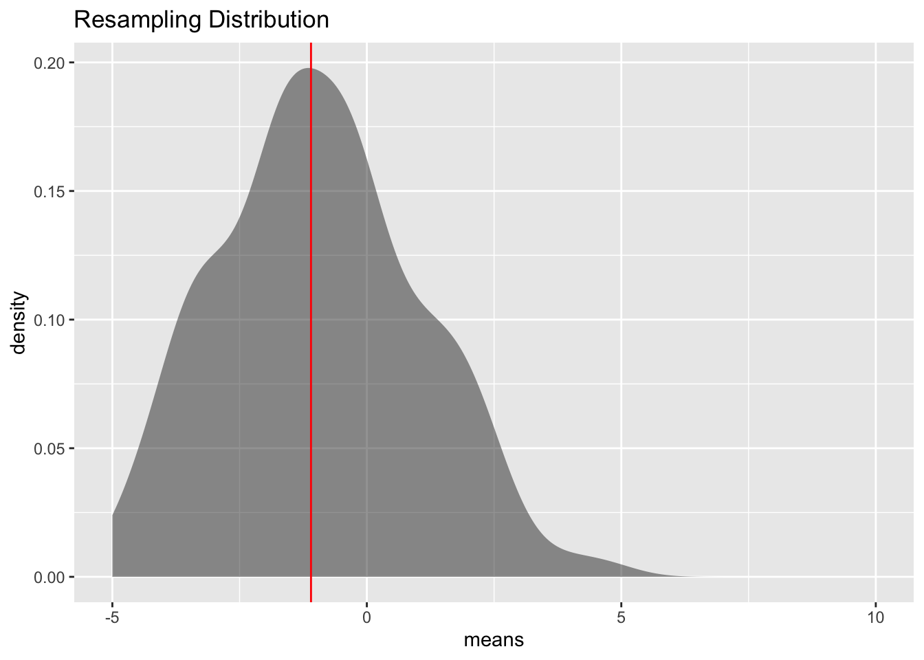

Resampling distribution of mean BMI with sample size 10, and measured sample mean. — Figure 7.1: Resampling distribution of mean BMI with sample size 10

Notice the sample mean from the resampling is very close to 0, so that means that the US BMI are not that different from the Australian BMI. There doesn’t seem to be enough evidence to show that the US BMI is different from the Australian BMI. One note, the sample size used here was 10 so you could see the sample, but really the sample size should be more than 100 for this method to be valid.

So this is one way to answer the question about if there is evidence to show a population mean is different from a value. This is actually the method that Ronald Fisher developed when he create all the foundation work that he did in statistics in the early 1900s. However, at the time, computers didn’t exist, so taking 100 resampling samples was not possible at that time. So other methods had to be developed that could be computed during that time. One method was developed by William (W.S) Gossett, a Chemist who worked for Guinness as their head brewer. Gossett developed a distribution called the Student’s T-distribution. His process was to use the sample standard deviation, $s$, as an approximation of $\sigma$. This means the test statistic is now $t=\frac{x-\mu}{\frac{s}{\sqrt{n}}}$. This new test statistic is actually distributed as a Student’s t-distribution, developed by W.S. Gossett. There are some conditions that must be made for this formula to be a Student’s t-distribution. These are outlined in the following theorem. Note: the t-distribution is called the Student’s t-distribution because that is the name he published under because he couldn’t publish under his own name due to his employer not wanting him to publish under his own name. His employer by the way was Guinness and they didn’t want competitors knowing they had a chemist/statistician working for them. It is not called the Student’s t-distribution because it is only used by students.

Theorem: If the following conditions are met

A random sample of size $n$ is taken.
The distribution of the random variable is normal.

Then the distribution of is a Student’s t-distribution with $n-1$ degrees of freedom.

Explanation of degrees of freedom: Recall the formula for sample standard deviation is $\sqrt{{\frac{\sum{x-\bar{x}}}{n-1}}}$. Notice the denominator is $n-1$. This is the same as the degrees of freedom. This is no accident. The reason the denominator and the degrees of freedom are both comes from how the standard deviation is calculated. First you take each data value and subtract $\bar{x}$. If you add up all of these new values, you will get 0. This must happen. Since it must happen, the first $n-1$ data values you have “freedom of choice”, but the nth data value, you have no freedom to choose. Hence, you have $n-1$ degrees of freedom. Another way to think about it is that if you five people and five chairs, the first four people have a choice of where they are sitting, but the last person does not. They have no freedom of where to sit. Only $n-1$ people have freedom of choice.

The Student’s t-distribution is bell-shape that is more spread out than the normal distribution. There are many $t$-distributions, one for each different degree of freedom.

Figure 7.2 is of the normal distribution and the Student’s t-distribution for df = 1, df = 3, df=8, df=30.

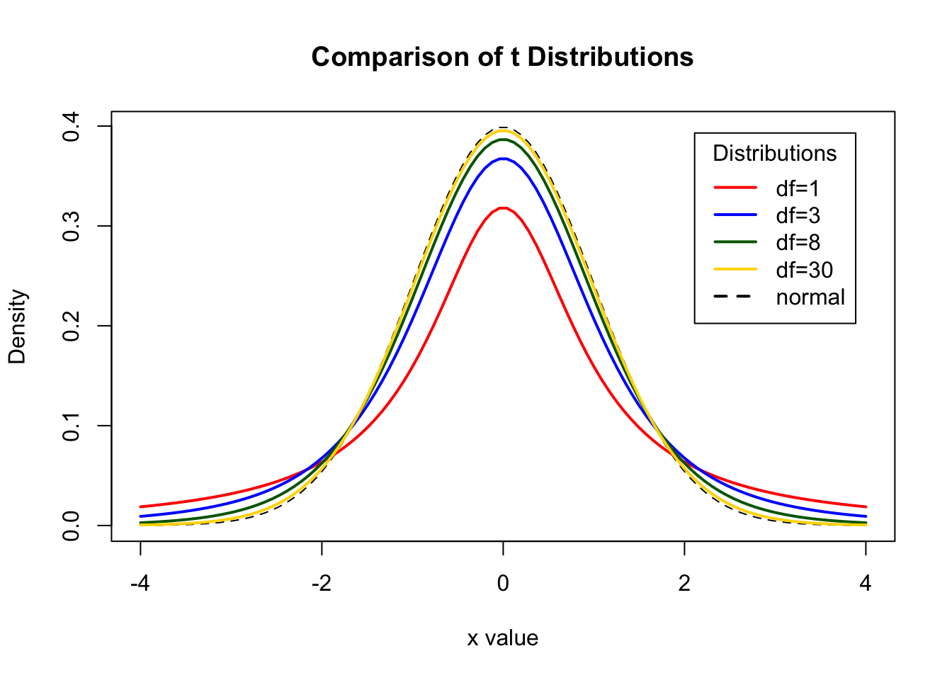
Student t distributions with different degrees of freedom and normal curve. — Figure 7.2: Typical Student t-Distributions

As the degrees of freedom increases, the student’s t-distribution looks more like the normal distribution.

To find probabilities for the t-distribution, again technology can do this for you. There are many technologies out there that you can use.

7.3.2 Hypothesis Test for One Population Mean (t-Test)

State the random variable and the parameter in words.

$x$ = random variable

$\mu$ = mean of random variable

State the null and alternative hypotheses and the level of significance

$H_o:\mu=\mu_o$ , where $\mu_o$ is the known mean

$H_a:\mu\ne\mu_o$, you can also use < or >, but $\ne$ is the more modern one to use.

Also, state your $\alpha$ level here.

State and check the conditions for a hypothesis test

State: A random sample of size $n$ is taken. Check: Describe the process taken to collect the sample.
State: The population of the random variable is normally distributed. Check: examine density graph and normal quantile plot. Note: The t-test is fairly robust to the condition if the sample size is large. This means that if this condition isn’t met, but your sample size is quite large, then the results of the t-test are valid.

Find the sample statistic, test statistic, and p-value

On rStudio, the command is

t.test(~variable, data=data_frame, mu=what_Ho_says)

Conclusion

This is where you write reject or fail to reject $H_o$. The rule is: if the p-value $<\alpha$, then reject $H_o$. If the p-value $\ge \alpha$, then fail to reject $H_o$

Interpretation

Note: if the conditions behind this test are not valid, then the conclusions you make from the test are not valid. If you do not have a random sample, that is your fault. Make sure the sample you take is as random as you can make it following sampling techniques from chapter 1. If the population of the random variable is not normal, then take a larger sample. If you cannot afford to do that, or if it is not logistically possible, then you do different tests called non-parametric tests or you can try resampling. The advantage fo resampling is that you don’t need to know the under laying distribution of the random variable.

7.3.3 Example: Test of the Mean Using One Sample T-test

A random sample of 50 body mass index (BMI) were taken from the NHANES Data frame Table 7.4. The mean BMI of Australians is 27.2 $kg/m^2$. Is there evidence that Americans have a different BMI from people in Australia. Test at the 5% level.

sample_NHANES_50<- sample_n(NHANES, size=50) 
knitr::kable(head(sample_NHANES_50))

Table 7.4: BMI of Americans
ID	SurveyYr	Gender	Age	AgeDecade	AgeMonths	Race1	Race3	Education	MaritalStatus	HHIncome	HHIncomeMid	Poverty	HomeRooms	HomeOwn	Work	Weight	Length	HeadCirc	Height	BMI	BMICatUnder20yrs	BMI_WHO	Pulse	BPSysAve	BPDiaAve	BPSys1	BPDia1	BPSys2	BPDia2	BPSys3	BPDia3	Testosterone	DirectChol	TotChol	UrineVol1	UrineFlow1	UrineVol2	UrineFlow2	Diabetes	DiabetesAge	HealthGen	DaysPhysHlthBad	DaysMentHlthBad	LittleInterest	Depressed	nPregnancies	nBabies	Age1stBaby	SleepHrsNight	SleepTrouble	PhysActive	PhysActiveDays	TVHrsDay	CompHrsDay	TVHrsDayChild	CompHrsDayChild	Alcohol12PlusYr	AlcoholDay	AlcoholYear	SmokeNow	Smoke100	Smoke100n	SmokeAge	Marijuana	AgeFirstMarij	RegularMarij	AgeRegMarij	HardDrugs	SexEver	SexAge	SexNumPartnLife	SexNumPartYear	SameSex	SexOrientation	PregnantNow
71857	2011_12	male	39	30-39	NA	White	White	College Grad	Married	more 99999	100000	5.00	9	Own	Working	73.4	NA	NA	175.7	23.80	NA	18.5_to_24.9	70	118	81	120	80	118	80	118	82	360.15	1.50	4.19	25	0.676	82	0.55	No	NA	Excellent	0	5	None	None	NA	NA	NA	7	No	Yes	2	More_4_hr	0_to_1_hr	NA	NA	Yes	2	52	NA	No	Non-Smoker	NA	Yes	19	No	NA	No	Yes	17	5	1	No	Heterosexual	NA
64282	2011_12	male	2	0-9	NA	Black	Black	NA	NA	10000-14999	12500	0.32	5	Rent	NA	12.2	88.4	NA	87.2	16.00	NormWeight	12.0_18.5	NA	NA	NA	NA	NA	NA	NA	NA	NA	NA	NA	NA	NA	NA	NA	NA	No	NA	NA	NA	NA	NA	NA	NA	NA	NA	NA	NA	NA	4	2_hr	1_hr	NA	NA	NA	NA	NA	NA	NA	NA	NA	NA	NA	NA	NA	NA	NA	NA	NA	NA	NA	NA	NA
69036	2011_12	male	76	70+	NA	Black	Black	9 - 11th Grade	Married	NA	NA	NA	7	Own	NotWorking	115.1	NA	NA	181.2	35.10	NA	30.0_plus	72	136	44	134	52	126	52	146	36	322.00	1.27	4.22	87	0.225	NA	NA	No	NA	Good	0	0	None	None	NA	NA	NA	8	No	No	NA	More_4_hr	0_hrs	NA	NA	No	2	36	No	Yes	Smoker	17	NA	NA	NA	NA	NA	NA	NA	NA	NA	NA	NA	NA
66845	2011_12	male	1	0-9	15	White	White	NA	NA	75000-99999	87500	3.15	9	Rent	NA	9.2	76.1	NA	NA	NA	NA	NA	NA	NA	NA	NA	NA	NA	NA	NA	NA	NA	NA	NA	NA	NA	NA	NA	No	NA	NA	NA	NA	NA	NA	NA	NA	NA	NA	NA	NA	5	NA	NA	NA	NA	NA	NA	NA	NA	NA	NA	NA	NA	NA	NA	NA	NA	NA	NA	NA	NA	NA	NA	NA
51745	2009_10	male	44	40-49	536	White	NA	College Grad	Married	more 99999	100000	3.97	8	Own	Working	84.6	NA	NA	182.0	25.54	NA	25.0_to_29.9	76	156	73	146	84	154	74	158	72	NA	0.98	4.42	85	1.574	NA	NA	No	NA	Good	0	5	None	None	NA	NA	NA	6	No	Yes	4	NA	NA	NA	NA	Yes	1	5	NA	No	Non-Smoker	NA	No	NA	No	NA	No	Yes	21	1	1	No	Heterosexual	NA
68833	2011_12	male	41	40-49	NA	Hispanic	Hispanic	High School	NeverMarried	NA	NA	1.61	3	Rent	Working	65.8	NA	NA	160.5	25.50	NA	25.0_to_29.9	62	116	76	114	68	114	76	118	76	210.53	1.37	3.88	199	1.005	NA	NA	No	NA	Fair	7	9	Several	None	NA	NA	NA	5	No	No	5	0_to_1_hr	0_hrs	NA	NA	Yes	8	52	No	Yes	Smoker	15	Yes	18	No	NA	No	Yes	13	2000	1	No	Heterosexual	NA

7.3.3.1 Solution

State the random variable and the parameter in words.

$x$ = BMI of an American

$\mu$ = mean BMI of Americans

State the null and alternative hypotheses and the level of significance

$H_o:\mu=27.2$

$H_a:\mu\ne 27.2$

level of significance $\alpha=0.05$

State and check the conditions for a hypothesis test

A random sample of 50 BMI levels was taken. Check: A random sample was taken from the NHANES data frame using r Studio
The population of BMI levels is normally distributed. Check:

(ref:sample-NHANES-50-density-cap) Density Plot of BMI from NHANES sample

gf_density(~BMI, data=sample_NHANES_50, title="Body Mass Index", xlab="Body Mass Index")
gf_qq(~BMI, data=sample_NHANES_50, title="Body Mass Index", xlab="Body Mass Index")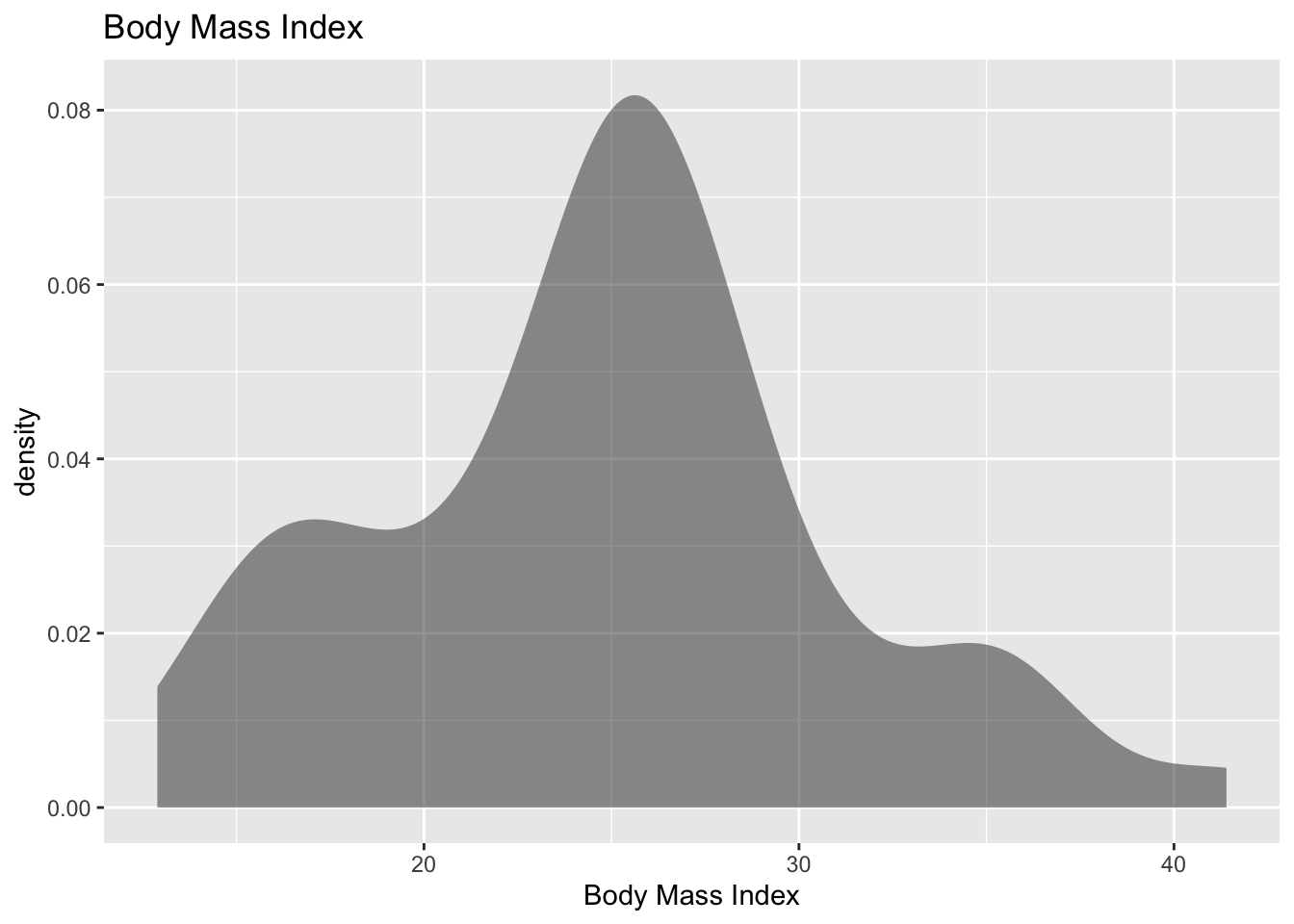

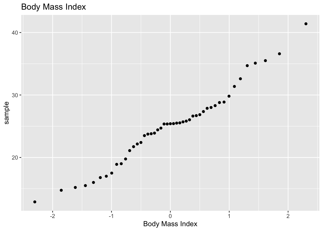
Density plot of BMI. Slightly right skewed — Figure 7.3: Density Plot of BMI from NHANES sample

The density plot looks somewhat skewed right and the normal quantile plot looks somewhat linear. However, there doesn’t seem to be strong evidence that the sample comes from a population that is normally distributed. However, since the sample is moderate to large, the $t$-test is robust to this condition not being met. So the results of the test are probably valid.

Find the sample statistic, test statistic, and $p$-value

On rStudio, the command would be

t.test(~BMI, data= sample_NHANES_50, mu=27.2)


    One Sample t-test

data:  BMI
t = -2.5245, df = 46, p-value = 0.0151
alternative hypothesis: true mean is not equal to 27.2
95 percent confidence interval:
 23.10436 26.73819
sample estimates:
mean of x 
 24.92128

The test statistic is the $t$ in the output, the sample statistic is the mean of $x$ in the output, and the $p$-value is the $p$-value is the output.

Conclusion

Since the $p$-value is not less than 5%, then fail to reject $H_o$.

Interpretation

There is not enough evidence to support that Americans have a different BMI from Australians.

Note: this is the same conclusion that was found when using resampling. So the two method could give similar conclusions.

7.3.4 Example: Test of the Mean Using One Sample T-test

In 2011, the average life expectancy for a woman in Europe was 79.8 years. The data in Table 7.5 are the life expectancies for all people in European countries (\“WHO life expectancy,” 2013). The Table 7.6 filtered the data frame for just males and just year 2000. The year 2000 was randomly chosen as the year to use. Do the data indicate that men’s life expectancy is different from women’s? Test at the 1% level.

Expectancy<-read.csv( "https://krkozak.github.io/MAT160/Life_expectancy_Europe.csv") 
knitr::kable(head(Expectancy))

Table 7.5: Life Expectancies for European Countries
year	WHO_region	country	sex	expect
1990	Europe	Albania	Male	67
1990	Europe	Albania	Female	71
1990	Europe	Albania	Both sexes	69
2000	Europe	Albania	Male	68
2000	Europe	Albania	Female	73
2000	Europe	Albania	Both sexes	71

Expectancy_male<- 
  Expectancy |>
  filter(sex=="Male", year=="2000") 
knitr::kable(head(Expectancy_male))

Table 7.6: Life Expectancies of males in European Countries in 2000
year	WHO_region	country	sex	expect
2000	Europe	Albania	Male	68
2000	Europe	Andorra	Male	76
2000	Europe	Armenia	Male	68
2000	Europe	Austria	Male	75
2000	Europe	Azerbaijan	Male	64
2000	Europe	Belarus	Male	63

Code book for data frame Expectancy

Description This data extract has been generated by the Global Health Observatory of the World Health Organization. The data was extracted on 2013-09-19 13:10:20.0.

This data frame contains the following columns:

year: year for life expectancies

WHO_region: World Health Organizations designation for the location of the country

country: country where the epectancies are from

sex: sex of the group that expectancies are calculated for

expect: average life expectancies of the different groups of the different countries.

Source http://apps.who.int/gho/athena/data/download.xsl?format=xml&target=GHO/WHOSIS_000001&profile=excel&filter=COUNTRY:*;SEX:*;REGION:EUR

References World Health Organization (WHO).

7.3.4.1 Solution

State the random variable and the parameter in words.

$x$ = life expectancy for a European man

$\mu$ = mean life expectancy for European men

State the null and alternative hypotheses and the level of significance

$H_o:\mu=79.8$

$H_a:\mu\ne79.8$

$\alpha=0.01$

State and check the conditions for a hypothesis test

State: A random sample of 53 life expectancies of European men in 2000 was taken.

Check: The data is actually all of the life expectancies for every country that is considered part of Europe by the World Health Organization in the year 2000. Since the year 2000 was picked at random, then the sample is a random sample.
State: The distribution of life expectancies of European men in 2000 is normally distributed.

Check:

gf_density(~expect, data=Expectancy_male, title="Life Expectancies of Males in Europe in 2000", xlab="Life expectancy")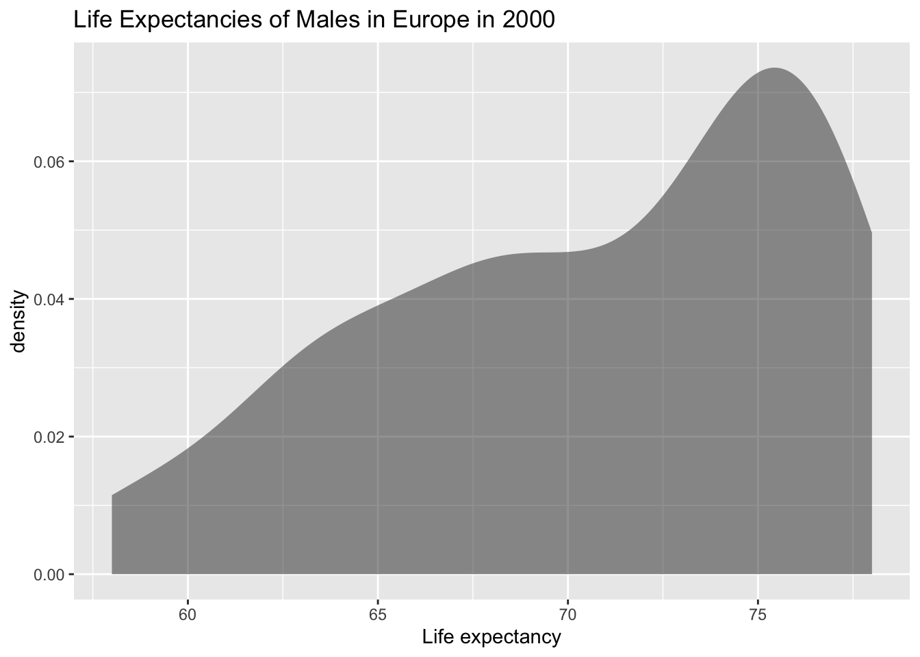

Density plot of life expectancy of males in Europe in 2000. — Figure 7.5: Density Plot of Life Expectancy of Males in Europe in 2000

gf_qq(~expect, data=Expectancy_male, title="Life Expectancies of Males in Europe in 2000")

quantile plot of life expectancy of males in Europe in 2000. — Figure 7.6: Quantile Plot of Life Expectancy of Males in Europe in 2000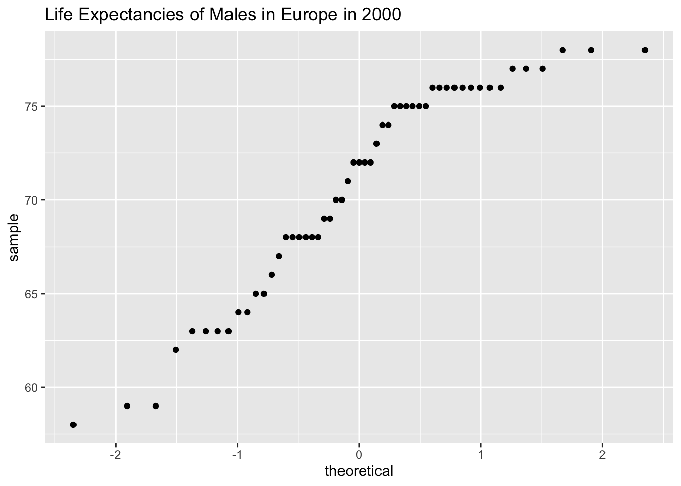

This sample does not appear to come from a population that is normally distributed. This sample is moderate to large, so it is good that the t-test is robust.

Find the sample statistic, test statistic, and $p$-value

On rStudio, the command is

t.test(~expect, data=Expectancy_male, mu=79.8)


    One Sample t-test

data:  expect
t = -11.733, df = 52, p-value = 3.145e-16
alternative hypothesis: true mean is not equal to 79.8
95 percent confidence interval:
 69.11930 72.23919
sample estimates:
mean of x 
 70.67925

Sample statistic is 70.68 years, test statistic is $t = -11.733$, and $p-value =3.14X10^{-16}$.

Conclusion

Since the p-value is less than 1%, then reject $H_o$.

Interpretation

There is enough evidence to support that the mean life expectancy for European men is different than the mean life expectancy for European women of 79.8 years.

Note: if you want to conduct a hypothesis test with $H_a:\mu>\mu_o$, then the rStudio command would be

t.test(~variable, data=Data_Frame, mu=number $H_0$ equals, alternative=“greater”)

If you want to conduct a hypothesis test with $H_a:\mu<\mu_o$, then the r Studio command would be

t.test(~variable, data=Data_Frame, mu=number $H_0$ equals, alternative=“less”)

7.3.5 Homework for One-Sample Test for the Mean Section

The Kyoto Protocol was signed in 1997, and required countries to start reducing their carbon emissions. The protocol became enforceable in February 2005. In 2004, the mean CO2 emission was 4.87 metric tons per capita. The Table 7.7 contains a random sample of CO2 emissions in 2010 (CO2 emissions (metric tons per capita), 2018). Is there enough evidence to show that the mean CO2 emission is different in 2010 than in 2004? Test at the 1% level.

Emission <- read.csv( "https://krkozak.github.io/MAT160/CO2_emission.csv") 
knitr::kable(head(Emission))

Table 7.7: CO2 Emissions (in metric tons per capita) in 2010
country	y1960	y1961	y1962	y1963	y1964	y1965	y1966	y1967	y1968	y1969	y1970	y1971	y1972	y1973	y1974	y1975	y1976	y1977	y1978	y1979	y1980	y1981	y1982	y1983	y1984	y1985	y1986	y1987	y1988	y1989	y1990	y1991	y1992	y1993	y1994	y1995	y1996	y1997	y1998	y1999	y2000	y2001	y2002	y2003	y2004	y2005	y2006	y2007	y2008	y2009	y2010	y2011	y2012	y2013	y2014	y2015	y2016	y2017	y2018
Aruba	NA	NA	NA	NA	NA	NA	NA	NA	NA	NA	NA	NA	NA	NA	NA	NA	NA	NA	NA	NA	NA	NA	NA	NA	NA	NA	2.8683194	7.2351980	10.0261792	10.6347326	26.3745032	26.0461298	21.4425588	22.0007862	21.0362451	20.7719362	20.3183534	20.4268177	20.5876692	20.3115668	26.1948752	25.9340244	25.6711618	26.4204521	26.517293	27.2007078	26.9477260	27.8950228	26.2295527	25.9153221	24.6705289	24.5075162	13.1577223	8.353561	8.4100642	NA	NA	NA	NA
Afghanistan	0.0460567	0.0535888	0.0737208	0.0741607	0.0861736	0.1012849	0.1073989	0.1234095	0.1151425	0.0865099	0.1496515	0.1652083	0.1299956	0.1353666	0.1545032	0.1676124	0.1535579	0.1815222	0.1618942	0.1670664	0.1317829	0.1506147	0.1631039	0.2012243	0.2319613	0.2939569	0.2677719	0.2692296	0.2468233	0.2338822	0.2106434	0.1833636	0.0961966	0.0850871	0.0758065	0.0686399	0.0624346	0.0566423	0.0527632	0.0407225	0.0372348	0.0378461	0.0473773	0.0504813	0.038410	0.0517440	0.0624275	0.0838928	0.1517209	0.2383985	0.2899876	0.4064242	0.3451488	0.310341	0.2939464	NA	NA	NA	NA
Angola	0.1008353	0.0822038	0.2105315	0.2027373	0.2135603	0.2058909	0.2689414	0.1721017	0.2897181	0.4802340	0.6082236	0.5645482	0.7212460	0.7512399	0.7207764	0.6285689	0.4513535	0.4692212	0.6947369	0.6830629	0.6409664	0.6111351	0.5193546	0.5513486	0.5209829	0.4719028	0.4516189	0.5440851	0.4635083	0.4372955	0.4317436	0.4155308	0.4105229	0.4417211	0.2881191	0.7870325	0.7262335	0.4963612	0.4758152	0.5770829	0.5819615	0.5743161	0.7229589	0.5002254	1.001878	0.9857364	1.1050190	1.2031340	1.1850005	1.2344251	1.2440915	1.2526808	1.3302186	1.253776	1.2903068	NA	NA	NA	NA
Albania	1.2581949	1.3741860	1.4399560	1.1816811	1.1117420	1.1660990	1.3330555	1.3637463	1.5195513	1.5589676	1.7532399	1.9894979	2.5159144	2.3038974	1.8490067	1.9106336	2.0135846	2.2758764	2.5306250	2.8982085	1.9350583	2.6930239	2.6248568	2.6832399	2.6942914	2.6580154	2.6653562	2.4140608	2.3315985	2.7832431	1.6781067	1.3122126	0.7747249	0.7237903	0.6002037	0.6545371	0.6366253	0.4903651	0.5602714	0.9601644	0.9781747	1.0533042	1.2295407	1.4126972	1.376213	1.4124982	1.3025764	1.3223349	1.4843111	1.4956002	1.5785736	1.8037147	1.6929083	1.749211	1.9787633	NA	NA	NA	NA
Andorra	NA	NA	NA	NA	NA	NA	NA	NA	NA	NA	NA	NA	NA	NA	NA	NA	NA	NA	NA	NA	NA	NA	NA	NA	NA	NA	NA	NA	NA	NA	7.4673357	7.1824566	6.9120534	6.7360548	6.4942004	6.6620517	7.0650715	7.2397127	7.6607839	7.9754544	8.0192843	7.7869500	7.5906151	7.3157607	7.358625	7.2998719	6.7460521	6.5193871	6.4278100	6.1215799	6.1225947	5.8674102	5.9168840	5.901775	5.8329062	NA	NA	NA	NA
Arab World	0.6457359	0.6874654	0.7635736	0.8782377	1.0030533	1.1705403	1.2781736	1.3374436	1.5522420	1.7986689	1.8103078	2.0037220	2.1208746	2.4095329	2.2858907	2.1967827	2.5843424	2.6487624	2.7623331	2.8636143	3.0928915	2.9302350	2.7231544	2.8165670	2.9813539	3.0618504	3.2844996	3.1978064	3.2950428	3.2566742	3.0169588	3.2366449	3.4154849	3.6694456	3.6743582	3.4240095	3.3283037	3.1455322	3.3499672	3.3283411	3.7038571	3.6079561	3.6046128	3.7964674	4.068562	4.1856773	4.2857192	4.1171475	4.4089483	4.5620151	4.6368134	4.5594617	4.8377796	4.674925	4.8869875	NA	NA	NA	NA

Code book for data frame Emission

Description Carbon dioxide emissions are those stemming from the burning of fossil fuels and the manufacture of cement. They include carbon dioxide produced during consumption of solid, liquid, and gas fuels and gas flaring.

This data frame contains the following columns:

country: country around the world

y1960-y2018: weighted averages of CO2 emission for the years 1960 through 2018 in metric tons per capita

Source CO2 emissions (metric tons per capita). (n.d.). Retrieved July 18, 2019, from https://data.worldbank.org/indicator/EN.ATM.CO2E.PC

References Carbon Dioxide Information Analysis Center, Environmental Sciences Division, Oak Ridge National Laboratory, Tennessee, United States.

The amount of sugar in a Krispy Kream glazed donut is 10 g. Many people feel that cereal is a healthier alternative for children over glazed donuts. The Table 7.8 contains the amount of sugar in a sample of cereal (breakfast cereal, 2019). Is there enough evidence to show that the mean amount of sugar in children’s cereal is different than in a glazed donut? Test at the 5% level.

Sugar <- read.csv( "https://krkozak.github.io/MAT160/cereal.csv") 
knitr::kable(head(Sugar))

Table 7.8: Nutrition Amounts in Cereal
name	manf	age	type	calories	protein	fat	sodium	fiber	carb	sugar	shelf	potassium	vit	weight	serving
100%_Bran	Nabisco	adult	cold	70	4	1	130	10.0	5.0	6	3	280	25	1	0.33
100%_Natural_Bran	Quaker_Oats	adult	cold	120	3	5	15	2.0	8.0	8	3	135	0	1	-1.00
All-Bran	Kelloggs	adult	cold	70	4	1	260	9.0	7.0	5	3	320	25	1	0.33
All-Bran_with_Extra_Fiber	Kelloggs	adult	cold	50	4	0	140	14.0	8.0	0	3	330	25	1	0.50
Almond_Delight	Ralston_Purina	adult	cold	110	2	2	200	1.0	14.0	8	3	-1	25	1	0.75
Apple_Cinnamon_Cheerios	General_Mills	child	cold	110	2	2	180	1.5	10.5	10	1	70	25	1	0.75

Code book for data frame Sugar

Description Nutritional information about cereals.

This data frame contains the following columns:

name: the cereal brand

manf: manufacturer

age: whether the cereal is geared towards children or adults

type: whether the cereal is considered a hot or cold cereal

calories: the number of calories in the cereal (number)

protein: the amount of protein in a serving of the cereal (g)

fat: the amount of fat a serving of the cereal (g)

sodium: the amount of sodium in a serving of the cereal (mg)

fiber: the amount of fiber in a serving of the cereal (g)

carb: the amount of complex carbohydrates in a serving of the cereal (g)

sugars: the amount of sugar in a serving of the cereal (g)

display shelf: what shelf the cereal is on counting from the floor

potassium: the amount of potassium in a serving of the cereal (mg)

vit: the amount of vitamins and minerals in a serving of the cereal (0, 25, or 100)

weight: weight in ounces of one serving

serving: cups per serving

Source (n.d.). Retrieved July 18, 2019, from https://www.idvbook.com/teaching-aid/data-sets/the-breakfast-cereal-data-set/ The Best Kids’ Cereal. (n.d.). Retrieved July 18, 2019, from https://www.ranker.com/list/best-kids-cereal/ranker-food

References Interactive Data Visualization Foundations, Techniques, Applications (Matthew Ward | Georges Grinstein | Daniel Keim)

A new data frame Table 7.9 will need to be created of just cereal for children. To create that use the following command in rStudio

Sugar_children<- 
  Sugar%>% 
  filter(age=="child") 
knitr::kable(head(Sugar_children))

Table 7.9: Nutrition Amounts in Children’s Cereal
name	manf	age	type	calories	protein	fat	sodium	fiber	carb	sugar	shelf	potassium	vit	weight	serving
Apple_Cinnamon_Cheerios	General_Mills	child	cold	110	2	2	180	1.5	10.5	10	1	70	25	1	0.75
Apple_Jacks	Kelloggs	child	cold	110	2	0	125	1.0	11.0	14	2	30	25	1	1.00
Bran_Chex	Ralston_Purina	child	cold	90	2	1	200	4.0	15.0	6	1	125	25	1	0.67
Cap’n’Crunch	Quaker_Oats	child	cold	120	1	2	220	0.0	12.0	12	2	35	25	1	0.75
Cheerios	General_Mills	child	cold	110	6	2	290	2.0	17.0	1	1	105	25	1	1.25
Cinnamon_Toast_Crunch	General_Mills	child	cold	120	1	3	210	0.0	13.0	9	2	45	25	1	0.75

The FDA regulates that fish that is consumed is allowed to contain 1.0 mg/kg of mercury. In Florida, bass fish were collected in 53 different lakes to measure the health of the lakes. The data frame of measurements from Florida lakes is in Table 7.10 (NISER 081107 ID Data, 2019). Do the data provide enough evidence to show that the fish in Florida lakes has different amounts of mercury than the allowable amount? Test at the 10% level.

Mercury<- read.csv( "https://krkozak.github.io/MAT160/mercury.csv") 
knitr::kable(head(Mercury))

Table 7.10: Health of Florida lake Fish
ID	lake	alkalinity	ph	calcium	chlorophyll	mercury	no.samples	min	max	X3_yr_standmercury	age_data
1	Alligator	5.9	6.1	3.0	0.7	1.23	5	0.85	1.43	1.53	1
2	Annie	3.5	5.1	1.9	3.2	1.33	7	0.92	1.90	1.33	0
3	Apopka	116.0	9.1	44.1	128.3	0.04	6	0.04	0.06	0.04	0
4	Blue_Cypress	39.4	6.9	16.4	3.5	0.44	12	0.13	0.84	0.44	0
5	Brick	2.5	4.6	2.9	1.8	1.20	12	0.69	1.50	1.33	1
6	Bryant	19.6	7.3	4.5	44.1	0.27	14	0.04	0.48	0.25	1

Code book for data frame Mercury

Description Largemouth bass were studied in 53 different Florida lakes to examine the factors that influence the level of mercury contamination. Water samples were collected from the surface of the middle of each lake in August 1990 and then again in March 1991. The pH level, the amount of chlorophyll, calcium, and alkalinity were measured in each sample. The average of the August and March values were used in the analysis. Next, a sample of fish was taken from each lake with sample sizes ranging from 4 to 44 fish. The age of each fish and mercury concentration in the muscle tissue was measured. (Note: Since fish absorb mercury over time, older fish will tend to have higher concentrations). Thus, to make a fair comparison of the fish in different lakes, the investigators used a regression estimate of the expected mercury concentration in a three year old fish as the standardized value for each lake. Finally, in 10 of the 53 lakes, the age of the individual fish could not be determined and the average mercury concentration of the sampled fish was used instead of the standardized value. ( Reference: Lange, Royals, & Connor. (1993))

This data frame contains the following columns:

ID: ID number

Lake: Name of lake

alkalinity: Alkalinity (mg/L as Calcium Carbonate)

pH: pH

calcium: calcium (mg/l)

chlorophyll: chlorophyll (mg/l)

mercury: Average mercury concentration (parts per million) in the muscle tissue of the fish sampled from that lake

no.samples: How many fish were sampled from the lake

min: Minimum mercury concentration among the sampled fish

max: Maximum mercury concentration among the sampled fish

X3_yr_Standard_mercury: Regression estimate of the mercury concentration in a 3 year old fish from the lake (or = Avg Mercury when age data was not available)

age_data: Indicator of the availability of age data on fish sampled

Source Lange TL, Royals HE, Connor LL (1993) Influence of water chemistry on mercury concentration in largemouth bass from Florida lakes. Trans Am Fish Soc 122:74-84. Michael K. Saiki, Darell G. Slotton, Thomas W. May, Shaun M. Ayers, and Charles N. Alpers (2000) Summary of Total Mercury Concentrations in Fillets of Selected Sport Fishes Collected during 2000–2003 from Lake Natoma, Sacramento County, California (Raw data is included in appendix), U.S. Geological Survey Data Series 103, 1-21. NISER 081107 ID Data. (n.d.). Retrieved July 18, 2019, from http://wiki.stat.ucla.edu/socr/index.php/NISER_081107_ID_Data

References NISER 081107 ID Data

The data frame Table 3.7 contains various variables about a person including their pulse rates before the subject exercised and after the subject ran in place for one minute. The mean pulse rate after running for 1 minute of females who do not drink is 97 beats per minute. Do the data show that the mean pulse rate of females who do drink alcohol is higher than the mean pulse rate of females who do not drink? Test at the 5% level.

Code book for data frame Pulse is below Table 3.7.

Create a data frame Table 9.2 that contains only females who drink alcohol. Then test the pulse after for woman who do drink alcohol to the known value for females who do not drink alcohol. To create a new data frame with just females who drink alcohol use the following command, where the new name is Females:

Females<- Pulse%>% filter(gender=="female", alcohol=="yes") 
knitr::kable(head(Females))

Table 7.11: Pulse Rates Before and After Exercise of Females who do drink Alcohol
height	weight	age	gender	smokes	alcohol	exercise	ran	pulse_before	pulse_after	year
165	60	19	female	yes	yes	low	ran	88	120	98
163	47	23	female	yes	yes	low	ran	71	125	98
173	57	18	female	no	yes	moderate	sat	86	88	93
179	58	19	female	no	yes	moderate	ran	82	150	93
167	62	18	female	no	yes	high	ran	96	176	93
173	64	18	female	no	yes	low	sat	90	88	93

The economic dynamism is an index of productive growth in dollars. Economic data for many countries are in Table 7.12 (SOCR Data 2008 World CountriesRankings, 2019). Countries that are considered high-income have a mean economic dynamism of 60.29.

Economics <- read.csv( "https://krkozak.github.io/MAT160/Economics_country.csv") 
knitr::kable(head(Economics))

Table 7.12: Economic Data for Countries
Id	incGroup	key	name	popGroup	region	key2	ED	Edu	HI	QOL	PE	OA	Relig
0	Low	al	Albania	Small	Southern_Europe	popS	34.0862	81.0164	71.0244	67.9240	58.6742	57	39
1	Middle	dz	Algeria	Medium	North_Africa	popM	25.8057	74.8027	66.1951	60.9347	32.6054	85	95
2	Middle	ar	Argentina	Medium	South_America	popM	37.4511	69.8825	78.2683	68.1559	68.6647	46	66
3	High	au	Australia	Medium	Australia	popM	71.4888	91.4802	95.1707	90.5729	90.9629	4	65
4	High	at	Austria	Small	Central_Europe	popS	53.9431	90.4578	90.3415	87.5630	91.2073	18	20
5	Low	az	Azerbaijan	Small	central_Asia	popS	53.6457	68.9880	58.9512	68.9572	40.0390	69	50

Code book for data frame Economics

Description These data represent commonly accepted measures for raking Countries on variety of factors which affect the country’s internal and external international perception of the country’s rank relative the to rest of the World.

This data frame contains the following columns:

id: Unique country identifier

incGroup: Income group: Low: GNI per capita < \$3,946, Middle: \$3,946 < GNI per capita < \$12,195, High: GNI per capita > \$12,196

key: unique 2-letter country code

name: Country Name

popGroup: Population Group: Small: Population < 20 million, Medium: 20 million < Population < 50 million, Large: Population > 50 million

region: Relative geographic position of the Country

key2: Country Group Classification Label: world: All countries, g7: G7, g20: G20, latin: Latin America & Caribbean, eu: European Union, centasia: Europe & Central Asia, pacasia: East Asia & Pacific, asean: Asean, sasia: South Asia, mideast: Middle East & North Africa, africa: Sub-Saharan Africa, bric: Brazil, Russia, India and China (BRIC)

ED: Economic Dynamism: Index of Productive growth in dollars (GDP/capita at PPP, Avg of GDP/capita growth rate over last ten years, GDP/capita growth rate over next ten years, Economic Dynamism: Manufacturing percent of GDP, Services percent of GDP percent (100=best, 0=worst).

Edu: Education/Literacy Rate (percent of population able to read and write at a specified age)

HI: Health Index: The average number of years a person lives in full health, taking into account years lived in less than full health

QOL: Quality of Life: Population percent living on < \$2/day

PE: Political Environment: Freedom house rating of political participation (qualitative assessment of voter participation/turn-out for national elections, citizens engagement with politics)

OA: Overall country ranking taking all measures into account.

Relig: Religiosity of the Country as a percent (%) of the population.

Source SOCR Data 2008 World CountriesRankings. (n.d.). Retrieved July 19, 2019, from http://wiki.stat.ucla.edu/socr/index.php/SOCR_Data_2008_World_CountriesRankings#SOCR_Data_-_Ranking_of_the_top_100_Countries_based_on_Political.2C_Economic.2C_Health.2C_and_Quality-of-Life_Factors

References SOCR Data 2008 World CountriesRankings, Amazon Web-Services World’s Best Countries.

Create a data frame that contains only middle income countries. Do the data show that the mean economic dynamism of middle-income countries is less than the mean for high-income countries? Test at the 5% level. To create a new data frame Table 7.13 with just middle income countries use the following command, where the new name is Middle_economics:

Middle_economics<- 
  Economics |> 
  filter(incGroup=="Middle") 
knitr::kable(head(Middle_economics))

Table 7.13: Economic Data for Middle income Countries
Id	incGroup	key	name	popGroup	region	key2	ED	Edu	HI	QOL	PE	OA	Relig
1	Middle	dz	Algeria	Medium	North_Africa	popM	25.8057	74.8027	66.1951	60.9347	32.6054	85	95
2	Middle	ar	Argentina	Medium	South_America	popM	37.4511	69.8825	78.2683	68.1559	68.6647	46	66
7	Middle	by	Belarus	Small	central_Asia	popS	51.9150	86.6155	66.1951	74.1467	34.0501	56	34
10	Middle	bw	Botswana	Small	Africa	popS	43.6952	73.4608	34.8049	50.0875	72.6833	80	80
11	Middle	br	Brazil	Large	South_America	popL	47.8506	71.3735	71.0244	62.4238	67.4131	48	87
12	Middle	bg	Bulgaria	Small	Southern_Europe	popS	43.7178	82.2277	75.8537	73.1197	73.1686	38	50

In 1999, the average percentage of women who received prenatal care per country is 80.1%. Table 2.18 contains the percentage of woman receiving prenatal care in a sample of countries over several years. (births per woman), 2019). Do the data show that the average percentage of women receiving prenatal care in 2009 (p2009) is different than in 1999? Test at the 5% level.

Code book for Data frame Fert_prenatal is below Table 2.18.

Maintaining your balance may get harder as you grow older. A study was conducted to see how steady the elderly is on their feet. They had the subjects stand on a force platform and have them react to a noise. The force platform then measured how much they swayed forward and backward, and the data is in Table 7.14 (Maintaining Balance while Concentrating, 2019). Do the data show that the elderly sway more than the mean forward sway of younger people, which is 18.125 mm? Test at the 5% level. Follow the filtering methods in other homework problems to create a data frame for only Elderly.

Sway <- read.csv( "https://krkozak.github.io/MAT160/sway.csv") 
knitr::kable(head(Sway))

Table 7.14: Sway (in mm) of Elderly Subjects
age	fbsway	sidesway
Elderly	19	14
Elderly	30	41
Elderly	20	18
Elderly	19	11
Elderly	29	16
Elderly	25	24

Code book for data frame Sway

Description How difficult is it to maintain your balance while concentrating? It is more difficult when you are older? Nine elderly (6 men and 3 women) and eight young men were subjects in an experiment. Each subject stood barefoot on a “force platform” and was asked to maintain a stable upright position and to react as quickly as possible to an unpredictable noise by pressing a hand held button. The noise came randomly and the subject concentrated on reacting as quickly as possible. The platform automatically measured how much each subject swayed in millimeters in both the forward/backward and the side-to-side directions.

This data frame contains the following columns:

Age: Elderly or Young

FBSway: Sway in forward/backward direction

SideSwayy: Sway in side to side direction

Source Maintaining Balance while Concentrating. (n.d.). Retrieved July 19, 2019, from http://www.statsci.org/data/general/balaconc.html

References Teasdale, N., Bard, C., La Rue, J., and Fleury, M. (1993). On the cognitive penetrability of posture control. Experimental Aging Research 19, 1-13. The data was obtained from the DASL Data and Story Line online database.